Why I Love the Beta Distribution (Part Two)

This is part two of my thoughts on a probability distribution that marketing research and analytics folks should get to know. Read the first installment here.

---

I’ve always thought that marketing researchers are frequentists while marketers are Bayesians. What does that mean? We collect data, summarize it, and stat test it as if there is no prior knowledge about the subject. That is the frequentist approach. Marketers are Bayesian in that they always approach new information with a prior expectation and then decide if the new information makes sense to them. Marketers rely heavily on prior beliefs. So how do we bridge the gap between signals we researchers send and what our internal clients receive?

‘B’ is for Bayes and for Beta

The Beta distribution lets us put some Bayesian in our game! The beta is the conjugate prior to the binomial so it becomes easy to incorporate prior knowledge into a study that is similar to one done before.

Let me start with a non-MR example. In 2018, Didi Gregorius, shortstop for the Yankees at the time, was hitting about .340 by the end of April. He won player of the month. Did you think he was going to hit 340 for the year? No. Why was 340 not the best estimate of his batting average for the full year? Because we had prior knowledge. The batting average in baseball for regulars is in the 260-270 range and few hit less than 215 nor more than 350. Didi had been about average through his career. We can fit a Beta distribution to these data and determine the two values for the parameters that best fit these facts. It happens to be alpha is 81 and beta is 219 (great piece on this here). Now, the cool thing about the beta as a conjugate prior to the binomial is that you just update it with successes and failures. So, in April, Didi had about 34 hits in 100 official at-bats. We add the 34 hits to alpha and the 66 outs to beta, and we update our parameters. The posterior mean for Didi’s batting average now becomes 287. (For the beta, the mean is really simple to calculate: It is alpha divided by alpha + beta.) So, no Sabermetricians would have thought that Didi would end the year with 340. Thanks to Bayesian math, 287 would be a better estimate. (He actually finished the year around 270.)

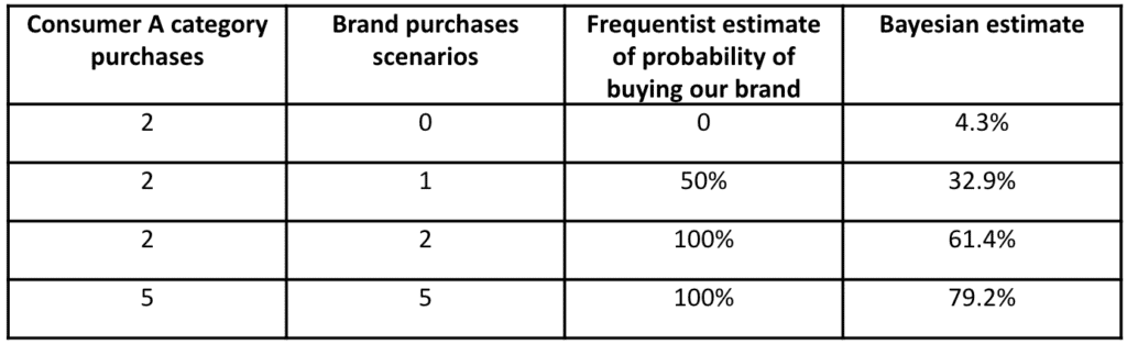
Now let me give you a real MR and analytics example. If we fit the beta to the distribution of probabilities of purchase for a brand with a 10% share and a 45% repeat rate, we will get something like alpha = .15 and beta = 1.35. So that beta distribution becomes our prior for a given consumer, we might be tracking via frequent shopper or receipt scanning data. Now, we want to classify this shopper in terms of likely loyalty to our brand but they only make two category purchases. If they bought us twice, do we think they are 100% loyal? If they bought us one out of two times, are they 50% loyal? Using the baseball Bayesian approach, we would make the following assessment.

Does it make sense that someone bought us twice in a row but only had a 61.4% probability of buying? Yes! There are 2.25 times as many consumers with a 61% probability of buying the 10 share brand vs. those with a 90% probability. So, if you work out the math, the posterior (likelihood x prior) for a 61.4% probability of buying is higher. Does it make sense that five out of five purchases for our brand give a higher posterior estimate of the probability of purchase than two out of two? Absolutely! More data, all consistent – but frequentists might not calculate a difference. Now we know a better way to segment individual shoppers from receipt scanning, household scanning, or frequent shopper data! Thank you, Beta Distribution!

One final cool thing about the Beta – Sometimes a researcher wants to present the median of data rather than the mean. Or you might want to say that 90% of the data will be in a certain range, rather than reporting a standard deviation. The confidence intervals around measures other than the mean are not that obvious. These measures, like the median, fall into a class of statistics called “order statistics”, and the probability distribution that is most universal for understanding how much variability there is in order statistics (like the median is)…wait for it…wait for it…the Beta Distribution! (You can bootstrap a data set or generate random numbers in Excel to prove this.)

So now you have it. The Beta is the right way to understand consumer purchase probabilities towards your brand, and it is critical for Bayesian thinking about percentages you might see in a given study where there is a prior track record. It is readily accessible via Excel, R, and Python. It even has stat testing usefulness for certain statistics. If I had a dog, I think I’d name him/her Beta!